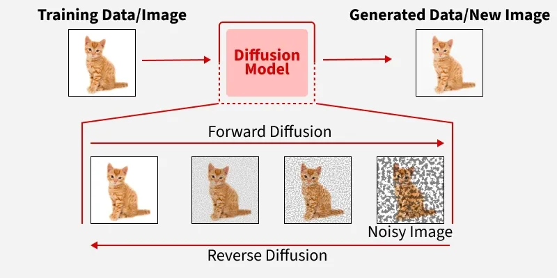
You’ve probably seen the absolute explosion of AI-generated art over the last few years. Whether it’s a hyper-realistic image of a dog riding a skateboard on Mars or a stunning digital painting: the internet is flooded with this stuff (especially my Instagram reels). The engine under the hood of all these incredible image generators (like Midjourney, DALL-E, Stable Diffusion and more recently NanoBanana) is something called a diffusion model. They work, quite literally, by taking an image of full of noise and slowly “denoising” it step-by-step until the image appears.
But why did diffusion completely take over the image generation world? The secret sauce is in how it handles complex distributions. Older image generators were tricky to train and often produced blurry or weirdly distorted results when asked to do something complicated. By design, classic neural networks are expected value approximators: they learn the mean of the distribution they are trying to model. This is why previously, when a face was image-generated, it looked very generic, almost like it was a blend of all the face images it has seen: that’s because it was, outputting the mean of all faces it has seen it’s the way to minimize the global loss during training.
Diffusion models, which work by taking random noise and slowly “denoising” it step-by-step, changed the game. They are stable to train, can capture fine detail, and (most importantly) they handle multiple valid options. If you ask a diffusion model for a picture of a house, it doesn’t just mathematically average every house it has ever seen into one blurry, generic blob. It commits to one distinct, high-quality sample.
Unpacking the Core Concept: What is a Diffusion Neural network?
To move from the specific application in robotics back to the broader architecture, we have to look at why Diffusion Neural Networks are fundamentally different from the “input-in, output-out” models we’ve used previously. In a standard deep learning model, the goal is to find a direct mapping function. If you want to generate a specific output, the network tries to jump from the input to the final result in a single forward pass. This usually works for one-to-one tasks, like classification (where there same input should lead to the same output: an image of a flower will/should always be classified as a flower). In one-to-many problems, like Generative AI, where ‘generating a flower’ has multiple correct outputs, the mapping mechanism of standard deep learning models falls apart.
The Score-Based Perspective Diffusion models change the objective from mapping to gradient following. Instead of learning what a “perfect” data point looks like, the network learns the score function, the gradient of the log-probability of the data.
Think of the data manifold (the collection of all valid, high-quality outcomes) as a series of mountain peaks. In this metaphor, the higher the elevation, the more “realistic” or “correct” the data is. The valleys below represent the infinite ways to produce noise or nonsensical results. Traditional Models tries to “teleport” from an input directly onto a peak. However, if the training data contains two different peaks (like a car turning left and a car turning right), the model’s math forces it to aim for the “average” coordinates between them. It tries to land in the middle of the two mountains, only to realize there is no ground there. Diffusion Models don’t try to leap to the summit in one go. Instead, it learns the score function: a mathematical “map of the slopes.” It studies the entire landscape and learns which way is “up” from any given point in the fog.
Handling the “One-to-Many” Problem The most significant advantage of this architecture is its inherent ability to handle one-to-many relationships. In standard regression, if the input could result in either or , the model’s loss function (like Mean Squared Error) will force it to predict . Diffusion networks avoid this because they are probabilistic samplers. They don’t predict a value; they model a distribution. By starting from a different noise each time, the same network can walk its way up different mountains (valid regions of the data). It treats the complexity of the real world not as noise to be averaged out, but as a landscape of valid peaks to be explored.
Speeding up Diffusion Models
Denoising Diffusion Probabilistic Models (DDPMs): The Stochastic Random Walk
DDPMs are the architecture that started the current generative AI boom. They operate as a Stochastic Differential Equation (SDE).
In a DDPM, the forward process destroys an image by injecting Gaussian noise step-by-step. The neural network is trained to estimate the “score” (the gradient of the log probability) to reverse this process.
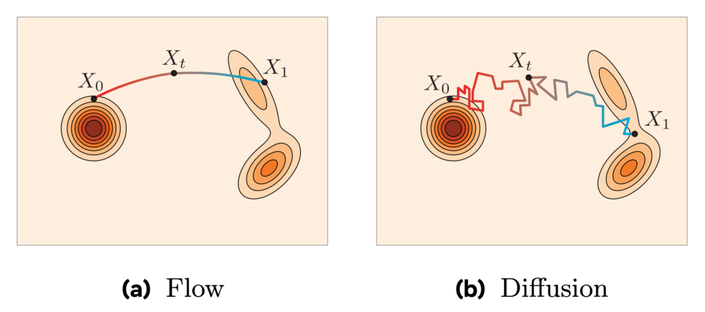
Because the noise injection is random (stochastic), the mathematical path from a clean image to pure noise is essentially Brownian motion, it is jagged, curved, and highly chaotic. When the neural network tries to reverse this process, it is forced to navigate this curved path.
If the mathematical “step size” it takes is too large, it will overshoot the curve and step off the data manifold, resulting in a distorted, unrecognizable image. Therefore, the model is trapped into taking hundreds or thousands of tiny steps (neural network evaluations) to safely traverse the curved probability space. This is what makes traditional diffusion so computationally expensive and slow.
Flow Matching: Deterministic Vector Fields
Flow Matching abandons the stochastic random walk entirely. Instead, it frames the generation process as an Ordinary Differential Equation (ODE). It treats the noise and the target data not as a sequence of corrupted images, but as two distinct distributions of particles.
Imagine a solid object made of sand (the data distribution). Now imagine you put a tiny explosive at the middle of it and detonate it (noising): it will become a cloud of sand grains (the Gaussian noise distribution). When accounting for air turbulence, the direction in which each grain of sand was blown away is noisy and unpredictable. On the other hand, if you ignore the turbulence of the air, every grain of sand has a distinct direction in which it was blown away. That is the main difference between diffusion models and flow matching models: the former model noisy and stochastic paths, the latter model clear paths.
Flow Matching trains a neural network to act as a Velocity Vector Field, denoted as . The network does not try to guess “how much noise to remove.” Instead, it looks at a particle at position at time and outputs a physical velocity vector: “Move this particle exactly in this direction, at this speed.”
Because Flow Matching uses ODEs, the trajectory from noise to data is deterministic, not random. More importantly, Flow Matching allows researchers to explicitly design the probability path. Instead of being forced to follow the chaotic curves of a DDPM, engineers can define simple, direct flows. The neural network simply learns to match this optimal vector field.
Rectified Flows: From Paths to Highways
If Flow Matching is the general framework for mapping one distribution to another using vector fields, Rectified Flows (and a closely related concept called Optimal Transport) are a specific, highly optimized application of that framework.
The core idea behind rectified flows is that the shortest distance between two points is a straight line. Rectified Flows force the paths between the noise particles and the data particles to be as straight and untangled as mathematically possible. If a vector field path is highly curved, you must take many tiny computational steps to follow it accurately. If you take a large step on a curved path, you shoot off into empty space (resulting in a distorted image).
Because the paths are enforced to be straight lines, the AI can take massive computational steps (using simple Euler integration) without flying off the path. This allows models like Stable Diffusion 3 (which uses Rectified Flows) to generate high-quality images in just 1 to 4 steps instead of 50.
Consistency Models: Skipping the Hike
Consistency Models take a completely different approach to speeding up the inference. Instead of trying to build a faster path or a straighter path, they try to build a teleporter. If you are anywhere on a specific path from noise to data, you shouldn’t have to follow the rest of the path to know where it ends.
The model is trained to enforce a strict mathematical rule: .
- Let be an image, and be the time-step (or noise level).
- If you are at time (very noisy) and time (slightly noisy) on the exact same trajectory, the network must output the exact same clean image ().
During training, the system looks at two adjacent points on a diffusion trajectory. It penalizes the neural network if it predicts a different final image for point A than it does for point B. The result ? Once trained, you can hand the model pure noise (time ), and it will evaluate the consistency function to instantly spit out the clean image (time ) in a single step. However, if you want higher quality, you can still chain a few steps together (e.g., jump from to , inject a tiny bit of noise, then jump to ) to refine the details.
Latent Diffusion: Shrinking the Universe
If standard diffusion models are the engine of generative AI, Latent Diffusion Models (LDMs) are what made that engine small enough to actually fit in your garage. Denoising a massive, high-resolution image pixel-by-pixel is computationally agonizing. LDMs bypass this by doing the heavy lifting in a compressed mathematical pocket dimension. If a neural network has to calculate the noise for every single pixel in a 4K image across 50 to 100 denoising steps, it requires a server farm of GPUs running at maximum capacity. It is simply too much data to process efficiently.
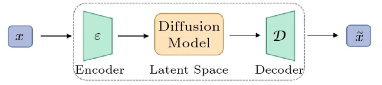
Instead of working directly in pixel space, the system uses an autoencoder to compress the image into a tiny, highly dense mathematical representation called the “latent space”. All of the noise injection and step-by-step denoising happens entirely within this compressed space.
Only at the very end, once the latent representation is perfectly clean, does a decoder blow it back up into the pixels we actually see on our screens. This clever architectural bypass reduced the compute cost so drastically that it allowed massive models (like Stable Diffusion) to run on standard consumer graphics cards, effectively democratizing generative AI overnight.
Beyond the Canvas: Diffusion Models Applications
The true power of the diffusion architecture lies in a simple, profound realization: in data science, “noise” is not just a grid of static pixels: noise can be anything. If you can represent a complex real-world concept as numbers, you can corrupt it with noise, and more importantly, you can train a diffusion model to clean it up. This makes diffusion a universal engine for mapping chaos back to structure, building directly on the foundational mathematics of nonequilibrium thermodynamics introduced in early denoising diffusion probabilistic models.
Escaping the 2D Canvas (Video and 3D)
The immediate next step was adding the dimensions of time and depth. When generating video, models like OpenAI’s Sora do not just generate a sequence of independent images, as that would result in a flickering, morphing mess. Instead, they treat the video as a spatiotemporal volume of noise encompassing width, height, and time. The model denoises the entire block simultaneously, ensuring that a character’s jacket stays the exact same shape and color from the first frame to the very last (https://openai.com/index/video-generation-models-as-world-simulators/).
Painting with Soundwaves
The exact same math used to draw a picture can be used to compose a symphony. Instead of denoising a photograph, audio diffusion frameworks like AudioLDM denoise a spectrogram, which is a visual representation of sound frequencies over time. By starting with visual static and slowly pulling out the distinct frequency bands, the model can generate high-fidelity sound effects, hyper-realistic text-to-speech, or fully arranged musical tracks (https://arxiv.org/abs/2301.12503).
The Scientific Frontier: Health and Material Science
This is where the technology leaves the media realm entirely and becomes a tool for scientific discovery. In biology, researchers are using models like RFdiffusion to invent entirely novel proteins that do not exist in nature. Instead of looking at pixels, the model looks at the 3D spatial coordinates of amino acids. It starts with a chaotic cloud of atomic noise and slowly denoises it into a stable, highly complex protein structure specifically designed to bind to a target, like a cancer cell or a virus (https://www.biorxiv.org/content/10.1101/2022.12.09.519842v1). We are effectively using diffusion to print custom medicine.
Discrete Text
Right now, autoregressive Large Language Models like ChatGPT rule the text generation world. They work by predicting the next word sequentially from left to right. But diffusion is coming for the throne. Researchers have been developing discrete diffusion models for text, such as Diffusion-LM. Instead of predicting one word at a time, these models start with an entire paragraph of masked, gibberish tokens and denoise the entire text at the exact same time (https://arxiv.org/abs/2205.14217). This allows the AI to perform complex, out-of-order reasoning and bidirectional editing, which is proving to be a massive leap for tasks like coding and logic.
The Physical World
Finally, if you can denoise an image, a soundwave, or a protein molecule, you can denoise physical motion. Robots do not output pixels; they output physical trajectories, including a sequence of motor commands, joint angles, and velocities over time. The conceptual leap here is incredibly elegant: we simply swap out the image for an action chunk. By starting with random, jagged motor noise, a diffusion policy can iteratively smooth it out until it becomes a highly precise, physically viable path for a robotic arm to follow (https://arxiv.org/abs/2303.04137).
Challanges and Limitations
Of course, no architecture is perfect, and diffusion models come with their own set of headaches. The most glaring issue is efficiency. Even with the “highways” of Rectified Flows, these models are computationally “heavy” compared to their autoregressive cousins (like ChatGPT). Because a diffusion model often has to process the entire output space at once rather than one token or pixel at a time, it struggles with long-context tasks.
In the world of text, for example, diffusion models still grapple with a “shallow dependency” problem, they are great at generating a coherent paragraph but can lose the plot over a long essay because they lack the deep, sequential reasoning of standard Transformers.
There’s also the controllability gap: while a diffusion model can give you a stunning forest, getting it to put a specific bird on a specific branch with 100% consistency every time is still a work in progress. For professionals in film or design who need “pixel-perfect” control, the “probabilistic” nature of diffusion can sometimes feel a bit too much like rolling dice.
Conclusion
Diffusion models have evolved from a clever mathematical trick for cleaning up grainy photos into a universal architect for complex data. By trading the “one-shot” guesswork of older models for a patient, step-by-step climb up the probability mountain, they’ve unlocked a level of creativity and precision that was previously the stuff of sci-fi.
Whether it’s shrinking the compute universe with Latent Diffusion, streamlining the path with Rectified Flows, or “teleporting” to the finish line with Consistency Models, the technology is moving at incredible speed. We are no longer just teaching machines to recognize our world; we are giving them a map of the “slopes” so they can help us build entirely new ones, from the pixels on your feed to the proteins in your medicine and the motions of the robots in our future.