In the previous post, we explored the rise of diffusion models in generative AI. The main takeaway was that instead of acting as simple “expected value” predictors, like classic neural networks do, diffusion models can map out complex, arbitrary distributions. This mathematical property is exactly why they are able to generate crisp, detailed images rather than averaging everything into a blurry blob.
The robot learning community is no stranger to the “average the correct answers” kind of behavior either, especially in imitation learning paradigms (our way of teaching robots from expert data). Think of an autonomous car going straight towards a pole: its training dataset has seen expert drivers avoid the pole by going right or by going left. Both methods would be completely valid. A standard neural network, however, doesn’t see two distinct options. It tries to find a mathematical compromise between the two, averages the steering angles, and drives straight into the pole (not a fun ride, if you ask me).
Recently, the robot learning community realized that the core strength of diffusion models could fix this. By allowing the AI to evaluate multiple valid possibilities, without averaging them into a disastrous middle ground, a diffusion policy can confidently commit to just one, higher quality path. Going from generating digital art to steering a physical robot might sound like a wild leap, but it actually solves a massive headache in traditional AI control.

How to leverage Diffusion Models for Robot Learning
Up until now we’ve been talking about the world of pixels and image generation. But robots don’t output pixels, they use physical trajectories. So, how do we take an architecture built for generating DALL-E images and use it to control a thousands of dollars worth robotic arm?
The conceptual leap, popularized in 2023 by researchers at Columbia and MIT (Chi et al.) and demonstrated in breakthrough systems like Stanford’s Mobile ALOHA,is actually surprisingly elegant: we simply swap out the “image” for an “action trajectory“. When watching these robots fluidly cook shrimp or fold laundry, the underlying mechanics are the same as DALL-E. Instead of denoising a 2D grid of RGB colors, the diffusion model denoises a sequence of motor commands over time, like joint angles, velocities, or the XYZ coordinates of a robotic gripper. The model still starts with pure, random noise, but as it iteratively refines that noise, it refines a smooth, physically viable path for the robot to follow. The mathematical process of “drawing a picture” becomes the exact same process as “planning a complex movement.”
While Diffusion Policy is incredibly powerful as a pure Imitation Learning tool (learning from human demonstrations), humans are imperfect, and our datasets don’t cover every edge case. To push a robot from ‘pretty good’ to ‘superhuman consistency’, researchers are increasingly taking these base Diffusion Policies and fine-tuning them using reinforcement learning (RL). The imitation learned diffusion model provides a highly capable, safe starting point, and RL provides the final polish to optimize for speed and error recovery.
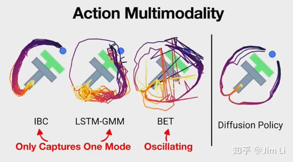
Results from “Diffusion Policy: Visuomotor Policy
Learning via Action Diffusion”, Cheng et al.
Imitation Learning for Diffusion Policies
The Secret Sauce: Action Chunking
At this point, you might be spotting a glaring problem: Latency. Diffusion takes multiple iterative denoising steps. If a robot needs to update its motors every 10 milliseconds, running a full diffusion loop which requires tens or houndreds of inferences for every single micro-movement is computationally impossible.
Enter Action Chunking. Instead of predicting a single action for the current millisecond (which assumes a strict Markovian state), the diffusion model predicts a ‘chunk’ of future actions, say, the next 64 steps or 2 seconds of movement all at once. The robot executes the first few steps of this chunk while the model simultaneously works on denoising the next overlapping chunk. This buys the model time to “think” while keeping the robot’s movement fluid.
Thinking in Sequences
When driving a car, you don’t consciously tell your hands to “turn the wheel 0.5 degrees for 10 milliseconds, then re-evaluate.” You plan sequences, like turning into the left lane over three seconds.
Traditional AI control did the opposite. Policies were typically markovian: the AI observes the current state and predicts a single action for that exact millisecond. Action chunking abandons this one-step-at-a-time convention. The neural network predicts a “chunk” of future actions all at once, say, the next 10 to 50 timesteps.
In the real world, however, the robot doesn’t execute the entire sequence blindly. It uses a receding-horizon approach: it starts executing the first few steps, but before finishing, it re-evaluates the environment and predicts a new chunk. This provides the benefit of a longer-term plan while remaining reactive to changes.
Why Predict the Future?
Predicting an entire trajectory at once solves several practical deployment issues.
First, it buys time. Vision-Language-Action (VLA) models are powerful, but computationally heavy. Forcing a large model to compute commands a hundred times a second leads to lag. Chunking allows the robot to execute the current sequence (or only part of it, if receding-horizon approach is applied) while the AI computes the next one in the background.
Second, chunking mitigates covariate shift. When a model predicts actions every millisecond, tiny errors compound. A slight miscalculation puts the robot in an unfamiliar position, causing a larger mistake on the next step. Committing to a sequence and checking the environment less frequently reduces these compounding feedback loops.
Finally, chunking forces the AI to learn meaningful representations. If an AI only predicts one millisecond ahead, it can cheat. Since physical motion is continuous, the AI can often just repeat its last motor command and minimize its loss. Predicting further into the future breaks this shortcut, requiring the model to understand the scene’s geometry and plan a coherent path.
Reinforcement Learning Finetuning
Imitation learning easily adopts chunking, but RL traditionally assumes that optimal policies only need to look one step ahead. Naively plugging action chunking into standard RL algorithms, which typically rely on Gaussian policies, causes performance to collapse.
Why RL Finetuning is beneficial
Imitation is a great start, but it has a few problems. First, the performance will only be as good as the data it is provided. Second, counterintuitively, if the data is taken from an expert is never wrong, then the policy we are training will never know how to recover from the mistakes (which are basically ensured in the world of statistical learners, such as neural networks).
Reinforcement learning overcomes these problems by actively exploring. Because RL is closed-loop and trial-and-error based, the robot inevitably makes sub-optimal moves during training. This forces the model into unfamiliar territory, directly solving the covariate shift problem we mentioned earlier. By actively experiencing its own mistakes, the AI maps out recovery trajectories, learning how to physically guide itself back to a successful path rather than just failing when things deviate from the human expert’s script.
Why RL Finetuning is hard
If action chunking and diffusion models are such a dream team for imitation learning, why can’t we just plug them into standard RL algorithms and call it a day? As it turns out, forcing a generative sequence model to learn via trial-and-error introduces three massive roadblocks: a fundamental misalignment in optimization goals and a clash between long-term sequence planning and RL’s traditional reactive nature.
One of the main problems is fundamental: diffusion models are inherently built to minimize a reconstruction loss, they are trained via maximum likelihood to make their generated outputs look exactly like the training data. Reinforcement Learning, on the other hand, doesn’t care about mimicking data (it doesn’t even have target data): it cares about maximizing a reward, and the optimal behavior to achieve that reward might not even exist in any fixed dataset.
The second hurdle is the clash between sequence planning and real-time reactivity. Standard RL algorithms are inherently Markovian, they operate on the assumption that the agent observes the current state, takes one immediate action, and repeats. Forcing RL to optimize an entire multi-step chunk of actions at once breaks this mathematical foundation. If the environment changes dynamically mid-chunk, a traditional RL critic doesn’t know how to evaluate or guide a sequence that is already halfway executed, causing the robot’s behavior to become fragile and slow to adapt.
The Diffusion-RL Mental Shift
To fully grasp how to apply RL to diffusion policies, a mental shift helps. We typically view Reinforcement Learning strictly as reward optimization. While true, RL is fundamentally a mathematical framework for optimizing any non-differentiable objective function.
Standard deep learning requires smooth, continuous math to calculate gradients and update weights. RL bypasses this constraint. It observes final outcomes and increases the probability of the network outputting actions that led to those results. We usually define these results as task success, but the target can be anything. For example, you could use RL to minimize a robot arm’s total energy consumption or maximize the physical smoothness of a trajectory.
With diffusion models, the optimization changes. We are not just updating the network to output a specific final action. We are optimizing the intermediate denoising steps the network takes to build that action.
How to Train Diffusion Policies with RL?
If Imitation Learning is about mimicking a human expert, Reinforcement Learning is about maximizing a mathematical reward. But merging these two paradigms presents a massive architectural challenge. Diffusion models were originally designed purely to reconstruct data distributions (like generating an image from noise), not to maximize a reward signal. Injecting RL into a diffusion model requires clever algorithmic engineering. Over the past few years, researchers have developed three primary ways to bridge this gap.
The first major breakthrough was Diffusion Q-Learning (DQL), introduced by Wang et al. (2022). In standard RL, a “Q-network” evaluates how good an action is. DQL turns the diffusion model into the actor and the Q-network into the critic. During inference, the diffusion model generates candidate action trajectories, and the Q-network scores them. During training, the gradients from the Q-network are backpropagated directly into the diffusion model’s denoising steps. Essentially, the diffusion model learns to warp its original data distribution to favor actions that the Q-network deems highly rewarding.
Another elegant approach is Reward-Guided Diffusion, which borrows directly from text-to-image models. In systems like Decision Diffuser or Planning with Diffusion, researchers bypass the need for a separate Q-network entirely. Instead, they treat the desired “reward” as a conditioning variable, much like a text prompt in DALL-E. You essentially prompt the model with a target return: “Generate a trajectory that achieves a high reward.” The denoising process is mathematically steered (using techniques like classifier-free guidance) toward the specific subspace of trajectories that historically led to success.
Most recently, the field has pushed toward online, actor-critic finetuning with algorithms like Diffusion-PPO (DPPO) (e.g., Zhuang et al., 2023 and related works). Proximal Policy Optimization (PPO) is the highly stable algorithm. DPPO adapts this for robotics by treating the entire, multi-step denoising chain as a single stochastic policy. By calculating the log-probabilities of the generated action sequences, DPPO can update the diffusion weights based on the actual physical rewards the robot receives in simulation. This allows the robot to actively explore and learn mistake-recovery behaviors in real-time, all while preserving the multi-modal expressiveness that makes diffusion models so powerful in the first place.
Predicting the Future with RL
Before Diffusion Policies arrived, the reinforcement learning community spent years trying to force AI agents to think in continuous sequences rather than single, isolated steps. Traditional RL is fundamentally Markovian: it looks at the current state, chooses one action, and waits for the next state. But physical robots require fluid, multi-step foresight. The journey to achieve this has been a constant game of trade-offs.
Early attempts focused on Hierarchical Reinforcement Learning (HRL), as formalized in Sutton’s Options framework. The idea was intuitive: split the brain. A high-level “manager” policy sets long-term goals (e.g., “pick up the cup”), while a low-level “worker” policy computes the immediate joint torques to execute it. However, training both levels simultaneously proved highly unstable; if the worker failed, the manager couldn’t learn effectively, creating a crippling chicken-and-egg training dynamic.
To bypass this instability, roboticists frequently turned to Movement Primitives (Schaal, 2006). Instead of predicting raw motor commands step-by-step, the AI outputs parameters for a mathematical curve that represents a full physical trajectory. While this guaranteed beautifully smooth robotic motions, these primitives were inherently rigid. They struggled to adapt in real-time to messy, unstructured environments where sudden corrections were necessary.
Later breakthroughs shifted toward Latent Space Planning, famously demonstrated by DeepMind’s MuZero. Instead of planning raw actions, the agent rolls out “mental simulations” of the future inside a compressed, learned representation of the world. While incredibly powerful for board games and discrete environments, mapping these abstract latent simulations back to the high-dimensional, continuous physics of a robotic arm remained computationally massive and prone to compounding errors.
This historical struggle highlights exactly why Action Chunking and Diffusion Policies have emerged as the potential grand unifiers. They allow the AI to directly output raw, continuous sequences of action (chunks) in one go, avoiding the unstable hierarchies of HRL, the mathematical rigidity of movement primitives, and the heavy mental simulations of latent planning.
The Bottlenecks and the Future
We have established that merging diffusion models, reinforcement learning, and action chunking creates a highly capable robotic brain. But we are not quite ready to put humanoid robots in every home.
The biggest roadblock right now is computational speed. Diffusion models are inherently slow because turning random noise into a crisp action plan requires dozens of mathematical steps. Earlier, we mentioned that action chunking ‘buys time.’ To be precise, chunking masks inference latency at the execution level, but the sheer computational weight (FLOPs) required to iteratively denoise trajectories remains a hard ceiling for physical robots.
This leads to the reaction problem. Chunking is fantastic for smooth, predictable tasks like folding clothes, but terrible for sudden, chaotic changes, like catching a falling glass. While dynamic chunk boundaries (where the AI learns to shift between long and short predictions) will help, the reality of modern deployment is hybrid architecture. To survive high-frequency chaos, Diffusion Policies are increasingly deployed strictly as high-level planners (running at slower rates, like ~10Hz), while battle-tested classical robotics techniques, such as low-level impedance controllers operating at 1000Hz, run underneath the AI to handle millisecond-to-millisecond physical stabilization.
While I can’t predict the future (unlike the dynamic latent models) I can only guess the community will be tackling these exact problems in the foreseeable future. To solve the speed issue, researchers are pushing towards faster math, exploring techniques like Consistency Models that aim to compress the long denoising process down to a single leap. To fix the reaction problem, a major milestone will be creating models that automatically determine their own chunk boundaries rather than relying on manual guessing and tuning. The AI will learn to predict long sequences when the coast is clear, and instantly switch to short, rapid predictions when the environment gets chaotic.
Conclusion
To wrap things up, we are looking at a fundamental shift in how we build brains for robots. For years, robot learning was stuck trying to squeeze messy, unpredictable real-world data into strict, deterministic, one-step boxes. The result was often an AI that compromised, averaged out the best solutions, and ended up crashing the car. Diffusion policies, paired with action chunking, flip that entire script.
By moving from rigid, single-step control to generative, sequence-based behavior, we are teaching robots to navigate the physical world the same way image generators navigate pixels. They no longer average their options or stumble forward millisecond by millisecond. Instead, they confidently pick one valid path and commit to a cohesive, multi-step plan, smoothly filtering out the noise along the way. We still have to iron out the latency and compute issues, but the resulting leap in physical dexterity is undeniable. The generative AI revolution has finally grown hands, and it is going to be exciting to see what it builds next.